
Ghost Signals: A Reverse Engineer’s Guide to Number Stations #2

In the previous episode, we spoke of number stations as “ghosts on the airwaves”: strange voices, mechanical tones, bursts of digital chatter. In Episode 2 is where we sharpen our tools and understanding, following the good old mindset of a reverse engineer, understanding the “assembly” of an RF (Radio Frequency) signal and what makes it a “signal” compared to pure noise and by establishing a reliable way to gather signals of interest (in our case Number Stations), which means learning about the different types of Number Stations (their Taxonomy) and how to acquire those signals.
The aim is, at the end of the post to be able to capture what we hear (acquire a signal), and recognize the spectral fingerprint of the most common signal types, with an especial focus on Number Stations.
Think of this as learning to spot “interesting” opcodes in a hex dump before attempting to reverse an entire program. Without this foundation, the more exotic signals will just look like noise. With it, they’ll begin to reveal structure.
Hunting the signals: where and how
Reverse engineers know the value of reconnaissance. In the Number Stations world, our main source will be Priyom.org, a community project that has logged years of Number Station activity. Their station schedule is the starting point for any real-world capture: UTC times, frequencies, and even intended target regions are listed in detail.
It’s worth spending a few words on what “target” means here, in our case those are the Number Stations. As we previously said, there entities are typically associated to shortwave transmissions from foreign intelligence agencies, embassies, military communication. The core advantage of a radio transmission, is that the recipient can be more or less anywhere in the world, receiving information without the need (which translates in fear of being discovered) to establish a link/connection with the emitter (over internet, classified or not you need to -establish- a connection). The additional advantage is that you are decoupled from “the internet” in case of disaster, what you are only left, to get in touch with the world and what is going on is…radio!
Number Station communications rely on a core aspect, the recipient must know the schedule, they must be at the right time, frequency and mode to be able to gather the message.
These elements are a solid reference points, which as reverse engineers (think about it…it’s no different from looking at the section names of your favorite PE to determine the packer used) represents a way to identify which specific Number Station we are talking about, allows us in other words, to create a taxonomy (humans knows by classifying). The official recognized Number Station taxonomy is the ENIGMA 2000 one (European Numbers Information Gathering and Monitoring Association). ENIGMA has a well defined prefix system:
E: English language voice broadcasts
G: German language voice broadcasts
S: Slavic language voice broadcasts
V: Voice broadcasts in all other languages
M: Morse code
F: Frequency-shift keying digital modes
P: Phase-shift keying digital modes
XP: Russian 7 digital modes
HM: Hybrids of analog and digital modes
Reference: Priyom.
These prefixes help listeners and researchers group similar transmissions and reduce confusion. Along with a letter, there is usually associated a number, some examples below:
V07: Known as Spanish Lady 000 000, this uses the “V” prefix (non-English/Slavic). It broadcasts three identical transmissions spaced 20 minutes apart, shifting slightly in frequency between runs.
S06: A Slavic-language station, “Russian Man” in voice, using USB + carrier mode. It fits under the “S” prefix.
As should expected, given the secretive nature of Number Station, the official references are kind of rare, G02 (known as Swedish Rhapsody) is one of those, for which there is a mention from the Polish Intelligence at the times of the Cold War. You will see in the document, the operators were given a frequency schedule along with some OPSEC directives (which are pretty interesting):
“
It is forbidden:
A} reception using receivers on grid power
B} reception using loudspeakers
C} reception using external antennas
…
“
If you want to stay up to date on the newest Number Station actors, ENIGMA 2000 Newsletter is definitely an up to date source to follow.
Now the core question, partially answered in the previous episode, how to listen, today?
We need to know the schedule, which gives us the frequency and the mode along with specific identifier (V07, G02, etc.). The identifier will tell us the approximate geographical location of the emitter, this is a core aspect we should keep into account because, if we are trying to gather a Number Station located in Asia, it’s way more likely to capture the signal, from an SDR located in approximate vicinity to the emitter. This means we have two main wait to collect number station transmissions:
With a common, physical SDR and antenna you can run at home. The basic setup can be quick and easy with an RTL-SDR dongle and free software such as SDR# or Gqrx.
Via one of the many WebSDR services freely available online. Below some examples.
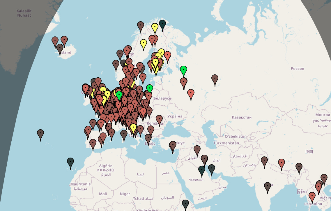
The famous Twente WebSDR in the Netherlands is a workhorse for European and Russian signals; Northern Utah and NA5B are excellent for Americas. For more choice there is http://rx.linkfanel.net/ with a practical map (see below) and WebSDR for more sources.
The steps to capture a number station, become pretty easy at this point:
Check the schedule, when a schedule says “E11, 1030 UTC on 12140 kHz USB,” you simply enter 12140 kHz, set the USB mode and watch the waterfall and listen, if you are interested in doing additional research, remember to record the .wav file.
As practical example, below you can find the capture of E07 as the prefix suggests it is a transmission in English, allegedly originated from Moscow, Russia in USB mode and located at 17456.00 kHz.
We can distinguish a triplet pattern of three digits, in this case “428” followed by a NULL (000).
Another example is M03 which as you now know, means Morse Code transmission, from the station 03, identified by the community as being of Polish origins. Observed for the first time in 1970 and currently still active. We will be leveraging an already Priyom recorded sample available here: https://priyom.org/media/117838/m03.ogg
Carrier, modulation, and modes, the grammar of signals
So what are we actually looking at? Let’s introduce two essential terms:
Carrier: The pure RF tone. If nothing modulates it, your waterfall shows a thin, steady line.
Modulation: It’s the process of imprinting the information on a carrier wave. Modulation changes the shape of the carrier wave to somehow encode the information (voice, data, etc.). A wave in essence can be seen as composed by three fundamental parameters:
Amplitude, varying it gives modulations such as AM/SSB.
Frequency, famous modulations are FM/FSK.
Phase, the most famous phase modulation is the PSK.
Read more:
Modulation can be divided into two main categories:
Analog, both the carrier and the signal are analog. The signal is superimposed on the carrier wave and has a continuous nature (means it can assume infinite values between two points). AM is an example of analog modulation. It can be seen as handwriting, with infinite gradations.
Digital, the carrier wave remains analog while the signal is digital, meaning that has a discrete nature (there are only two values possible, 0 and 1). FSK (Frequency Shifting Key) is a form of digital modulation. On the contrary of “handwriting” the states are fixed and can be more easily quantified.
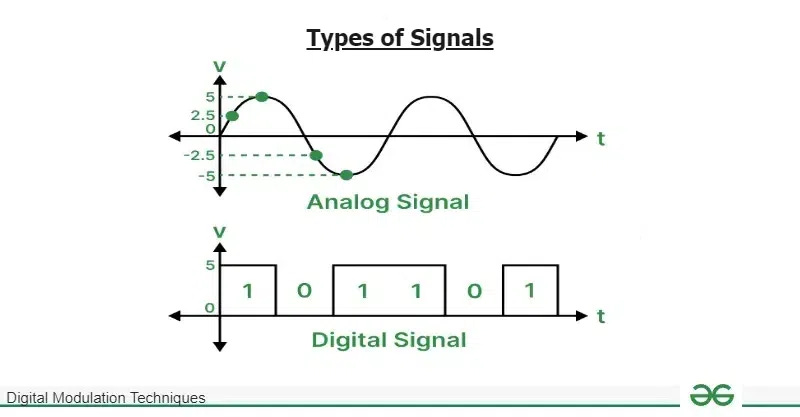
Credits: https://www.geeksforgeeks.org/electronics-engineering/digital-modulation-techniques/
In presence of an analog modulation, amplitude/frequency/phase of the carrier wave will change with respect to the amplitude of the signal. While, in a digital modulation signal, the three core components of the wave changes will shift between two or more discrete values. This process is called “Shift Keying” (the “SK” you see in modulations such as FSK, PSK, etc.). As trivia moment, older WiFi used a form of PSK (Phase Shifting Key) modulation type, while the most modern instances like WiFi-6 uses OFDM (Orthogonal Frequency-Division Multiplexing) where the signal is divided into “sub-carriers” making it more resistant to interference…but that’s another topic :)
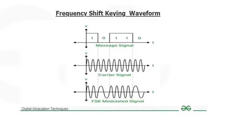
Credits & read more: Digital Modulation Techniques.
Reading waterfalls: patterns as opcodes
We got a few samples (the .wav files) and the foundations of what a Signal, in its essence is, let’s now try to look at the waterfall (spectrogram) which visualizes frequency over time, think of it as as a time-frequency disassembly. More technically we will be looking into an STFT (Short-time Fourier transform) which in very simplistic terms, tells us which frequencies exists at each moment in time.
Credits: STFT
We can therefore leverage an STFT representation (for easiness, a waterfall spectrum) to visualize and measure how a signal looks like.
Waterfall/Spectrum Visual Analysis
In this section we will be leveraging two samples, E07 and M03 to conduct a spectrographic analysis, this will be the occasion to cover additional topics associated to signal processing and signal analysis and create a process to structurally analyze a waterfall plot.
E07
The next waterfall we have is the E07 recording. Before jumping straight into the analysis, it’s important to have the rudiments of how an AM. Amplitude Modulation (AM) is a method of transmitting information by varying the amplitude (strength) of a carrier wave in proportion to the audio signal being sent. When you modulate a carrier wave with an audio signal, you create three components:
The carrier frequency: the original unmodulated wave
Upper Sideband (USB): frequencies above the carrier
Lower Sideband (LSB): frequencies below the carrier
In conventional AM broadcasting (like AM radio stations), all three components are transmitted. However, this is inefficient because:
The carrier contains no information (just power)
Both sidebands contain the same information (mirror images)
Single Sideband (SSB) solves this by transmitting only one sideband and suppressing the carrier and the other sideband. This provides:
More efficient power usage (all power goes into the information)
Narrower bandwidth (half the spectrum space)
Better range and clarity
We have therefore “two-half” signals, those are classified as:
USB (Upper Sideband): transmits only frequencies above the carrier
LSB (Lower Sideband): transmits only frequencies below the carrier
Check SSB for more.
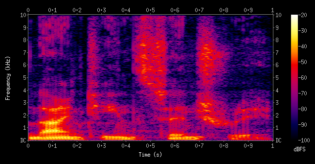
Here we have finally our sample’s spectrogram.
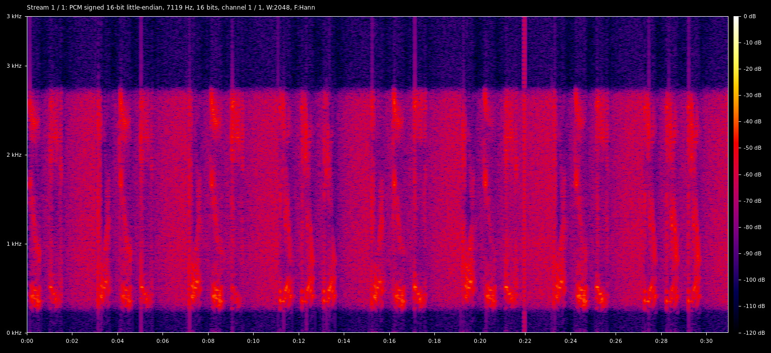
Let’s go step by step.
Time Axis (x-axis: 0 to 0.30 s): The plot covers 30 s per major tick emission, during which there is a steady modulated (see the huge “redish” band?) signal.
Frequency Axis (y-axis: 0 to 4 kHz): This is the baseband audio bandwidth post-demodulation (we did set our SDR receiver, already to the correct mode in this case), consistent with single-sideband (SSB) or vestigial sideband modes on HF, where the full signal occupies ~3-4 kHz. No evidence of wider bandwidth (e.g., >8 kHz for FM broadcast).
Energy Distribution: Dominant energy is concentrated in the lower half (0-2 kHz), with a steep roll-off above 2 kHz (fading from red to purple/blue). Peak PSD exceeds -10 dB in 200-800 Hz bands, dropping to -60 dB by 3 kHz. This envelope matches human speech acoustics.
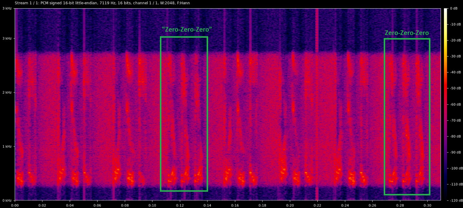
Temporal Behavior: Energy bursts are quasi-periodic, with ~50-100 ms on/off cycles (the vertical “redish” columns at ~0.05 s, 0.12 s, 0.18 s). No continuous broadband noise floor (the level of background noise in a signal or recording system that is present when no useful signal is being recorded) elevation (which would fill the plot in yellow/orange, as in white noise or interference). Instead, we observe discrete “events” which suggest modulated symbols or phonemes. We can go a step further on that, by observing the Vertical Striations and Harmonics but first is worth clarifying what an harmonic is. In short: harmonics are signal components whose frequencies are positive integer multiples of a signal’s fundamental frequency. For example, if a signal’s fundamental frequency is 50 Hz, its second harmonic is at 100 Hz, its third at 150 Hz etc. Back to the analysis, within the red/yellow bursts the faint vertical lines (50-200 Hz spacing) suggest an harmonic structure, with a rapid onset (<10ms) ans a 30-50ms sustained plateau, this is a typical trait of voiced speech, if you like the topic, this happens due to the vocal tract excitation, a nice starting point to go more in depth is: Spectrographic Analysis of Speech, an complete analysis would reveal additional features of the voice (the presence of what is likely the fundamental frequency + low harmonics suggests a male voice). As additional “trivia” from the vertical striations we can clearly spot the NULL (Zero-Zero-Zero) element, below an annotated version (notice how we have two NULL, one at ~0:12 sec, which you can match with the above audio of E07 and one toward the end).
We can at this point rule out a number of possible modulations:
Not CW/Morse: No isolated narrow vertical lines (<50 Hz wide) persisting across time, CW would appear as thin, constant-frequency streaks.
Not Pure Tone or Carrier: Absence of a single dominant horizontal band.
Not Digital (PSK/FSK etc.) : No characteristic paired lines (PSK) or shifted carriers (FSK ~500 Hz apart) with rectangular envelopes.
Not FM/NBFM: FM would show symmetric sidebands around a carrier, with flatter temporal envelopes.
In conclusion we have a “voice speech” artifacts, no symmetric sidebands around the carrier wave and no digital artifacts, this asymmetry points out to a possible AM/USB mode. USB matches with E07 Priyom classification.
M03
Let’s start from M03, which stands for Morse code (CW = Continuous Wave). CW uses an OOK (On-Off Keying) modulation, which very simply consists in turning on and off the carrier wave, which creates the famous dashes and dots that composed the Morse alphabet. The bandwidth of the CW signal is approximately 4 Hz per WPM (words per minute), more on Sigwiki-CW.
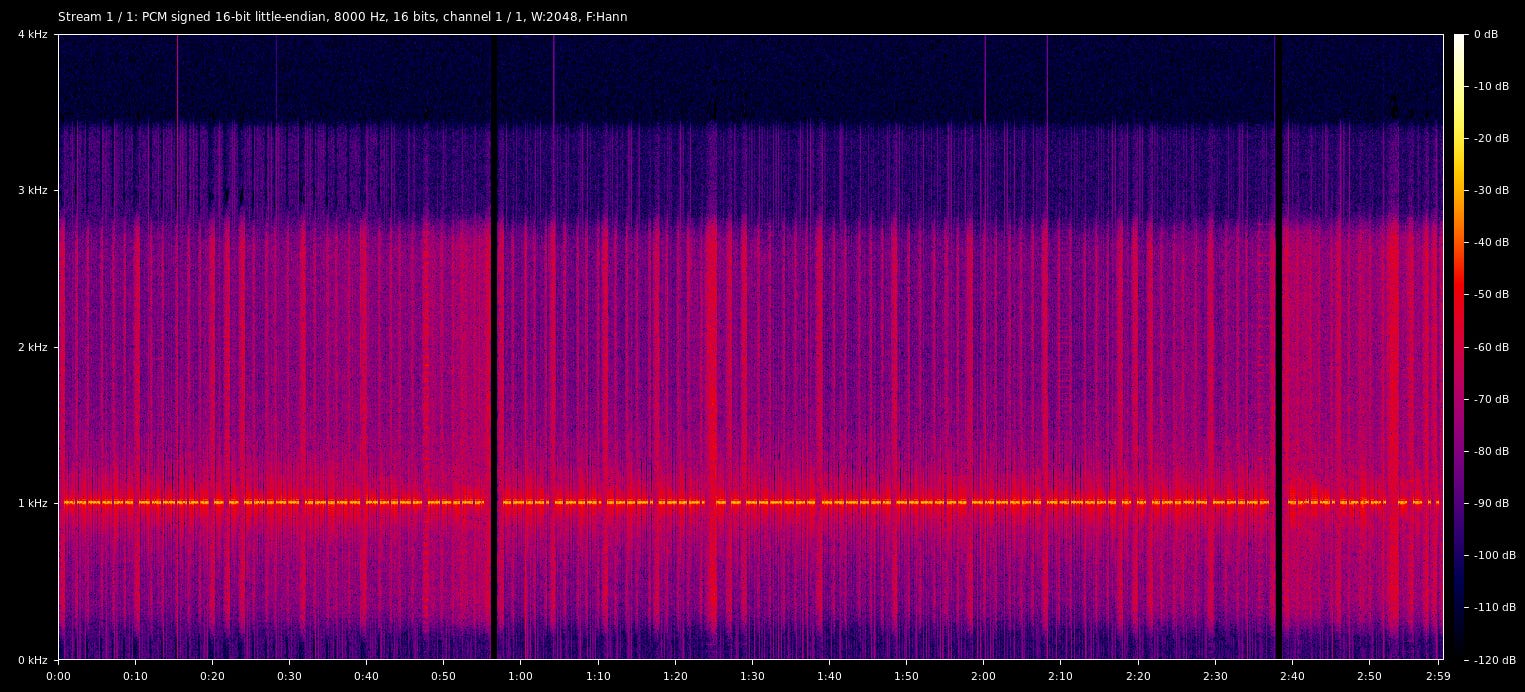
Time Axis (x-axis: 0 to 2.59 mins): : The horizontal span covers a total duration of approximately 2 minutes and 59 seconds, with a well defined and repetitive rhythm. The carrier wave shows an ON/OFF (can we spot any clue here? ;)) progression. We can see clear repetitive impulsive bursts, alternating short (about 1.8-3.6 s) and medium (6-12 s) red verticals, with consistent ~12-24 s gaps. The regular pattern hints an automated sequencing rather than manual variability (a human artifact is not that razor sharp precise in layman’s terms), similarly to the short term, in the long one (full sample timespan) we can see a repetitive pattern that keeps going.
Frequency Axis (y-axis: 0 to 4 kHz): The plot displays a standard 4 kHz baseband audio spectrum, typical of post-demodulation output from an SDR receiver (yep as before we knew and tuned already to the known modulation). Dominant signal energy is confined to a narrow ~80-120 Hz band. Such a narrow, centered concentration suggests a single-tone or low-deviation modulation.
Intensity Scale (color: blue to red/yellow, -120 dB to 0 dB): Broad dynamic range emphasizes sharp peaks (red > -20 dB) over quiet voids (blue < -110 dB). Clean scaling without bleed (in other words, we have sharp peaks).
Energy Distribution: Extremely narrow (~80-120 Hz wide), centered ~700-800 Hz, with >95% power in sub-kHz region and rapid drop-off above 1 kHz (purple/blue < -70 dB).
Vertical Striations and Keying: Uniform vertical red dashes/dots with crisp transitions. We observe a stric timing, with two recurring elements, one “short” (rings a bell? dots?) and one longer (dashes?).
What we can rule out so far?
Not Pulsed Markers (Radars does that): Irregular phrases (allow me the term) vs. fixed pulse repetition.
Not MCW (Modulated CW): Absent audio sidebands (be aware CW is not the only alternartive, we can have MCW aka Modulated Continuous Wave).
Conclusions indicates that, over a ~3 mins observation period we have a signal of cyclic nature (that’s what rhythm is), this is further reinforced by the carrier wave (see how it goes -cleary- ON and OFF) the evidences gathered so far indicates an OOK (On-Off Keying).
CW / Morse Code, as probably everybody knows is used to transmit text, obviously in the field of Number Stations, the text is encrypted, therefore you get sequences of numbers and/or letters. CW is still used for a number of advantage it has, the extremely narrow carrier makes it suitable for long range transmissions and there is still a world of communications you can catch with a simple WebSDR or a cheap shortwave radio. How to the code it? here you go! Morse Code Decoders Software Directory
All the spectrum visualizations have been carried via Spek a free Linux application.
Whats next
As you noticed, signal analysis is quite a vast field, with a pletora of modulations, some of those are pretty common (AM, FM, CW etc.) yet there are pillars that is worth knowing, such as RTTY, what FSK/PSK is.
Should we always do a long thorough visual analysis? Nope.. there are some great resources we can check first, such as:
Reddit - Signal Identification
..and yes there are other cool ways to identify a signal nowadays, like Torchsig (A PyTorch Signal Processing Machine Learning Toolkit ) but this will be matter for future posts ;)